In this blog post, we want to answer the question:

As the title suggests, this blog post directly responds to Sander Dieleman’s blog post ‘Diffusion is spectral autoregression’ which I really enjoyed. I spoke to many researchers in the community about it, and it prompted me to think about the relationship between Large Language Models (LLMs) and diffusion models, and why each excels on different tasks and data modalities. This blog post is accompanied by a paper titled ‘A Fourier Space Perspective on Diffusion Models’ together with my co-authors at Microsoft Research Cambridge that I cite at the very end of the post, and from which the majority of content is drawn from. Even though the focus of this blog post is slightly different, I will directly paraphrase from it where convenient. I begin by summarising Sander’s post from my perspective, qualitatively using exactly his argument, but trying to augment it with my own discussion and some new figures. Up front, I want to explain the notion of approximate spectral autoregression, because it is central to Sander’s post.

We will understand this definition carefully in the now following first part of this blog post.

Background: DDPM Diffusion is approximate spectral autoregression

Diffusion models are the state-of-the-art model on data such as images, videos, proteins and materials. Whether it is Stable Diffusion v1/v2 or Imagen for text-to-image generation [1], [2], Sora for producing high-resolution videos of impressive fidelity [3], RFdiffusion or BioEmu for generating protein structures [4], [5], or MatterGen for synthesising inorganic materials [6]: diffusion models serve as the workhorse for these modalities, and autoregressive models (LLMs), which excel on text, seem to not be able to compete with them (at least at present, and when considering all aspects including computational efficiency). – Why is that? What do these modalities have in common which renders diffusion models the superior model?

Data modalities where diffusion excels follow a Fourier power law.

In my quest to answer this question, I found Sander Dieleman’s blog post ‘Diffusion is spectral autoregression’, which very convincingly discussed an argument I was lingering on for a while: the modalities where diffusion models work well—images, videos, audio, proteins, materials and others—share the property of a decaying signal variance in Fourier space. Low-frequency components have orders of magnitude higher signal variance (and magnitude) than high frequencies (see the figure below).

Let’s understand this carefully. Say we have a natural image (Figure 1, [left]). Its pixels are the coefficients over a standard basis (${\mathbf{e}}_1=(1,0,0,0,\dots {)}^T,{\mathbf{e}}_2=(0,1,0,0,\dots {)}^T,\dots$): each pixel defines the constant value the image takes in a spatially-constrained part of the image. If we take this image and compute its discrete Fourier transform (DFT), we obtain a representation that contains the same information, but now in Fourier space (Figure 1, [right]). This Fourier image has the same dimension as the pixel image, but its coefficients are complex-valued (rather than real-valued), and we here plot their magnitude.

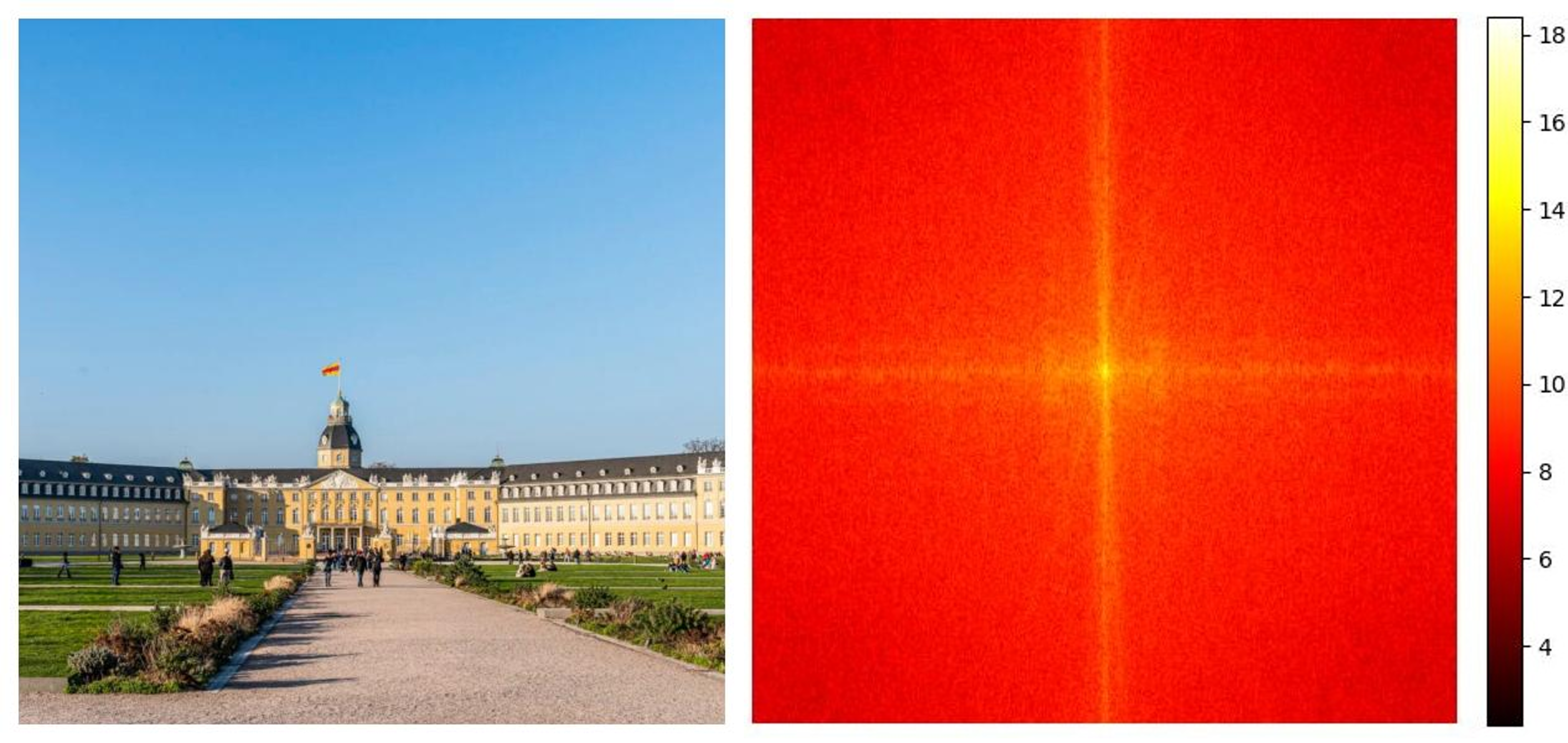
We now apply the DFT to a dataset of images, and compute the variance per dimension, assuming all images have equal dimensions (and we otherwise interpolate them), illustrated in the heatmap in Figure 2. Standard DFT libraries sort the coefficients in a way that those coefficients corresponding to low frequencies are in the centre and those corresponding to high frequencies are towards the edges/corners of the Fourier-transformed image. We can immediately see that low-frequency components have a significantly larger signal variance than high-frequencies. That’s not a new finding by the way: Field and van der Schaaf et al. observed this phenomenon in image data over 30 years ago [7], [8] (and that’s just the oldest sources I could find in related work, it was probably known for longer), [9] viewed it recently in the context of diffusion models. But where does this notion of frequency come from?

Each coefficient in Fourier space corresponds to basis functions which are a mixture of sines and cosines of different frequency. To see this, we can write the DFT in 2D (considering an image with one channel as an example) as $$X[k,\ell ]=\sum _{m=0}^{N-1}\sum _{n=0}^{N-1}x[m,n]\cdot e^{-2\pi i\left(\frac{km+\ell n}{N}\right)}.$$ where $X[k,\ell ]$ is a dimension of our Fourier-transformed image and $x[m,n]$ is a pixel (coefficient in the standard basis). Using Euler’s formula, we can write the DFT as $$\underset{\text{Fouriercoefficient}}{\underbrace{X[k,\ell ]}}=\sum _{m=0}^{N-1}\sum _{n=0}^{N-1}\underset{\text{pixel}}{\underbrace{x[m,n]}}\underset{\text{Fourier basis function}}{\underbrace{[\cos \left(2\pi \left(\frac{km+\ell n}{N}\right)\right)-i\sin \left(2\pi \left(\frac{km+\ell n}{N}\right)\right)]}}$$ In pixel space, each tuple $(m,n)$ indexes one unique pixel. We can for instance achieve this by (arbitrarily) indexing from the top-left corner of the image, but there is no notion of frequency in pixel space. In Fourier space, however, higher values of $k$ and $\ell$ correspond to basis functions, sine and cosine functions, which vary faster, which have a higher frequency.

We now want to make our life a little bit easier and sort the Fourier coefficients $X[k,\ell ]$ in one dimension from low to high frequency (of the corresponding basis function), which is easier to handle if we have data of different sizes, such as 1D (audio), 2D (image) and 3D data (video, protein density maps) data. To do so, we start at the centre of our Fourier space representation, and walk in a spiral towards the edges. More precisely, we sort them by Manhattan distance of the indices $(k,\ell )$ from the centre of the Fourier representation at (0,0) (which naturally works for 1D and 3D data, too). If we apply this sorting to the dimension-wise variances in Fourier space in Figure 2, we get a 1D tensor of variances.

In Figure 3 ¹ , we look at these (one-dimensional) sorted signal variances for image, video, audio and protein datasets, respectively. Since dimension-wise signal variances can sometimes vary a lot between neighbouring dimensions and we are mainly interested in the overall trend, we are actually plotting a running average of the signal variance. – And there we have it: the signal variance decreases rapidly with increasing frequency. Not just for images as we’ve already seen above, but also for other modalities which diffusion models really work well for.

Fourier power law data under a DDPM forward diffusion process

What happens if we now add noise to data which exhibits this Fourier power law property? In the DDPM forward process, we add white noise to a data item (say an image), meaning that each dimension of the noise in Fourier space has equal variance. More specifically, we obtain a noisy data item ${\mathbf{x}}_t$ as $${\mathbf{x}}_t=\underset{\text{signal}}{\underbrace{\sqrt{{\bar{\alpha }}_t}{\mathbf{x}}_0}}+\underset{\text{noise}}{\underbrace{\sqrt{1-{\bar{\alpha }}_t}\mathit{ϵ}}},\mathit{ϵ}\sim \mathcal{N}(0,\mathbf{I}).$$ Equivalently, we can view the forward process in Fourier space, applying the DFT operator $\mathbf{F}$, obtaining (by linearity of $\mathbf{F}$) $$\begin{array}{rl}{\mathbf{y}}_t:=\mathbf{F}{\mathbf{x}}_t& =\mathbf{F}(\sqrt{{\bar{\alpha }}_t}{\mathbf{x}}_0)+\mathbf{F}(\sqrt{1-{\bar{\alpha }}_t}\mathit{ϵ})\\ & =\underset{\text{signal }\mathbf{s}}{\underbrace{\sqrt{{\bar{\alpha }}_t}\mathbf{F}{\mathbf{x}}_0}}+\underset{\text{noise }\mathbf{n}}{\underbrace{\sqrt{1-{\bar{\alpha }}_t}\mathbf{F}\mathit{ϵ}}}.\end{array}$$ The vector ${\mathbf{y}}_t$ is our Fourier-transformed image, a grid of complex-valued coefficients. We call the left part signal, and the right part noise (in Fourier space). Furthermore, we can easily show that $\mathbf{n}\sim \mathcal{CN}(\mathbf{0},\mathbf{F}(1-{\bar{\alpha }}_t)\mathbf{I}{\mathbf{F}}^{†})=\mathcal{CN}(\mathbf{0},(1-{\bar{\alpha }}_t)\mathbf{I}),$ where ${\mathbf{F}}^{†}$ is the adjoint of $\mathbf{F}$, and $\mathcal{CN}(\cdot )$ is a complex normal distribution. As time increases, ${\bar{\alpha }}_t$ becomes small converging to 0, and the noise in Fourier space becomes large. Conversely, the signal is scaled converging to $\mathbf{0}$ as time increases.

Why can we simply introduce the operator $\mathbf{F}$ you might ask. Isn’t there a fundamental difference if we add noise in image space versus in Fourier space? – Since $\mathbf{F}$ is invertible, there is a one-to-one correspondence between a DDPM forward process in image space and its corresponding forward process in Fourier space. So a forward process in image space, where we might actually perform the noising computation, can always be equivalently viewed in Fourier space.

Now let’s bring it all together in Figure 4 ² . We have a signal variance (green) which features the Fourier power law and is in addition decreasing (scaled down) with diffusion time, and we have white noise whose variance increases with diffusion time (blue). We observe that as we add more and more noise in the forward process, the high-frequencies are dominated by that noise first, in the sense that the signal plus the noise is almost equal to the noise for those frequencies, since the noise is orders of magnitude larger.

A quantitative measure which captures this notion formally is the Signal-to-Noise Ratio (SNR). The SNR (red line in Figure 4) is defined as $$\mathsf{SNR}(f)=\frac{\mathrm{Var}[s]}{\mathrm{Var}[n]},$$ where $f(s,n)=s+n$ and $s$ and $n$ are coordinates of $\mathbf{s}$ and $\mathbf{n}$ in our definition for ${\mathbf{y}}_t$ above. Here, we can directly obtain it from the plot by dividing the signal (green) by the noise (blue line) at all timesteps.

The inductive bias of the forward diffusion process

The SNR is central to analysing the inductive bias of diffusion models [14] . It directly governs which frequencies are changing when in the forward process. Now you might ask: what does this imply for the backward process? Intuitively, the backward process reverses the forward process. If it does, the forward process induces a hierarchy into the generative process: low frequencies are generated before high frequencies [15]. But since the backward process is learned, does it actually reverse or mirror the forward process? What if it learned a short cut? Does the frequency hierarchy of the forward process truly govern the hierarchy in which frequencies are generated in the reverse process?

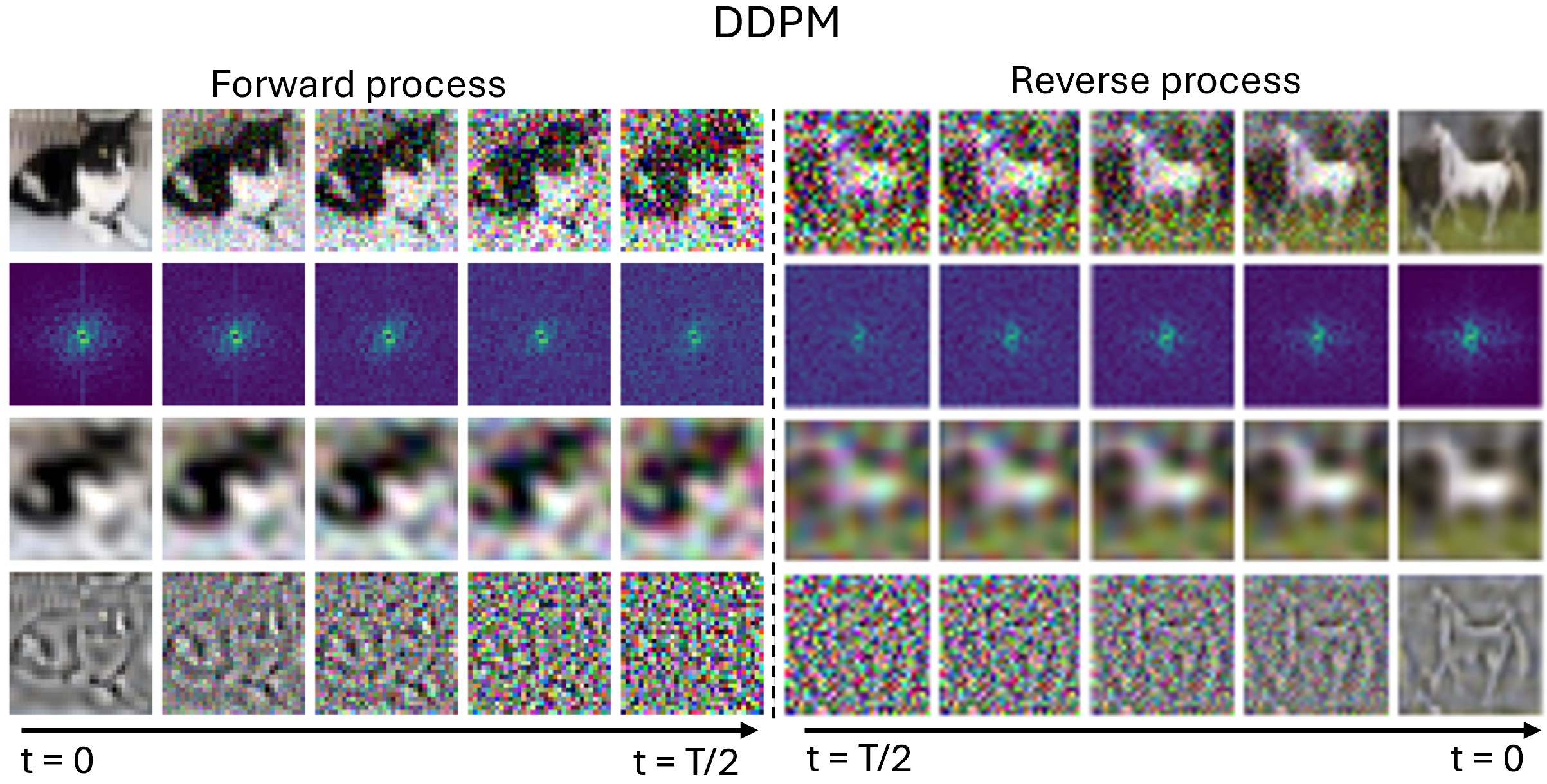
The answer is yes, and pretty accurately so. One way to see this is by looking at high- and low-pass filtered images at the beginning and end of the forward and reverse process of a diffusion model trained with DDPM (Figure 5). We observe that the high pass-filtered image [4th row] quickly becomes indistinguishable from noise and all high-frequency information is gone, while in the low-pass filtered image [3rd row], the low-frequency information remains for much longer: it is still recognisable at $t=T/2$ (half-way through the forward process going $t=0$ to $t=T)$. The reverse process mirrors this: low-frequency information is already visible at $t=T/2$ (half-way through the reverse process going $t=T$ to $t=0$), while high-frequency information is added mostly during the latter half of the reverse process. For completeness, rows 1 and 2 show the (unfiltered) image in pixel and Fourier space, respectively. This illustrates precisely the intuition of ‘approximate spectral autoregression’ in DDPM, and we will later contrast this with a hierarchy-free diffusion model.

A second, quantitative perspective is by considering the SNR (here in units of decibel, $10\times {\log }_{10}(\cdot )$) in the forward and the reverse process, illustrated across time (x-axis) and per frequency (y-axis) in Figure 6. The SNR of the forward process is straightforwardly computed as a Monte Carlo estimate of variance of signal and noise in our equation for ${\mathbf{y}}_t$ above and then plugging these into the definition of the SNR (we could also compute it analytically, but we decided to sample instead, which is closer to what we actually compute during training). Since we don’t know the noise in the reverse process, we cannot do the same for the reverse process.

As a proxy, we proceed as follows: we denoise an image step-by-step, starting from pure Gaussian noise ${\mathbf{y}}_T$. In each diffusion step, we predict the clean image ${\hat{\mathbf{y}}}_0$, and by reparameterizing obtain the added noise $$\widehat{\mathit{ϵ}}=\frac{1}{{\sqrt{1-\alpha }}_t}({\mathbf{y}}_t-\sqrt{{\bar{\alpha }}_t}{\hat{\mathbf{y}}}_0).$$ Now, we estimate a proxy for the SNR in the reverse process as $$\stackrel{\mathsf{~}}{\mathsf{SNR}}({\mathbf{y}}_{t-1})=\frac{\sqrt{{\bar{\alpha }}_{t-1}}\mathrm{Var}[{\hat{\mathbf{y}}}_0]}{\sqrt{1-{\bar{\alpha }}_{t-1}}\mathrm{Var}[\widehat{\mathit{ϵ}}]},$$ where the variance is computed over a batch of sample trajectories. Obviously, this approach is prone to approximation error of our neural network predicting the clean image: the estimate ${\hat{\mathbf{y}}}_0$ is not the ‘true’ clean image. But assuming the neural network is trained well (and we use it at training convergence), it is a quantity measuring something like SNR in the reverse process.

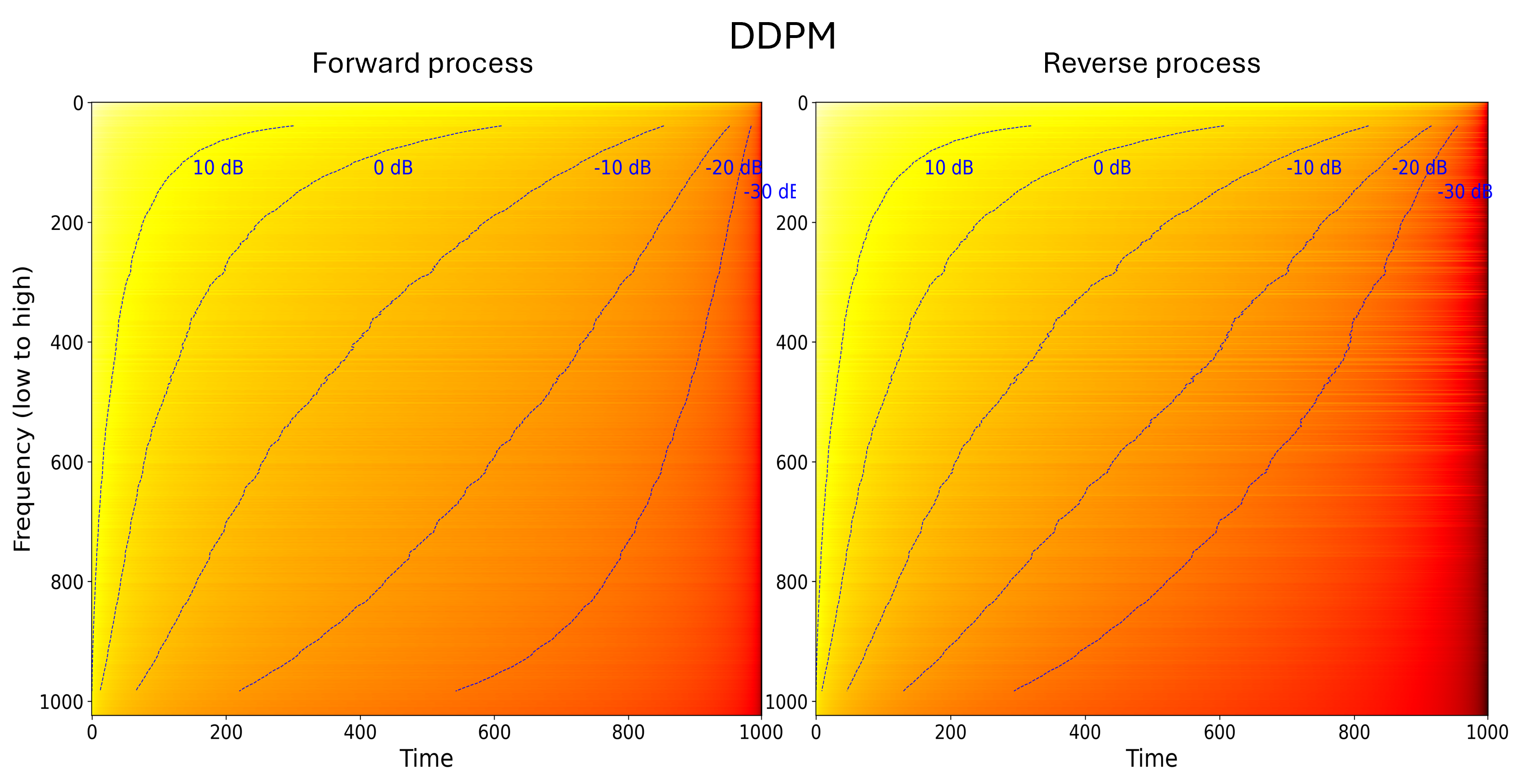
The reverse process hence indeed follows a frequency hierarchy during generation, an approximate spectral autoregression as Sander framed it pointedly, generating low frequencies first, then high frequencies conditional on the low frequencies.

A concluding comment on this first part and the term approximate spectral autoregression: An autoregressive model (say an LLM) factors the data distribution as $p(\mathbf{y})=p(y_1,y_2,\dots ,y_D)=\prod _{d=1}^{D}p(y_d\mid y_1,y_2,\dots ,y_{d-1})$, i.e. each dimension is generated one-by-one, conditional on all previously generated dimensions. In diffusion models, however, the number of diffusion steps $T$ is typically much smaller than the number of dimensions $D$ (aka. pixels aka. frequencies aka. tokens) in the data, $T\ll D$. The diffusion model hence cannot generate frequencies ‘one-by-one’, and rather generates multiple frequencies at the same time. We can also see this in the heatmap above: the active frequencies are those which have not yet reached the maximum SNR at a given timestep, and the active time interval overlaps between frequencies [15]. The order or hierarchy of the frequencies is hence ‘soft’, and this is what Sander expresses with the classifier ‘approximate’ before ‘spectral autoregression’. In fact, this overlap of frequencies is possibly what renders diffusion models computationally efficient!

Does the inductive bias of the forward process matter?

As we have seen, DDPM has implicitly chosen the order in which frequencies are generated, namely—with lots of overlap—from low to high frequency. This occurred almost by coincidence: we have chosen a simple, white noise distribution for the forward process, and just because the data happens to feature the Fourier power law, high frequencies are dominated by noise first. If the data distribution had a different spectral profile, the same frequency hierarchy would not appear. – The natural question to ask is: Is this hierarchy or ordering of frequencies necessary? Were we just extremely lucky (or perhaps smart) choosing white noise on images (and other modalities) which happens to be a beneficial choice? Or do diffusion models still work if we do not have this hierarchical structure in Fourier space?

Token hierarchy in LLMs.

With an empirical hat on, of course the order in which we process frequencies should matter. In autoregressive LLMs, for example, it matters and directly impacts performance if we generate a piece of text left-to-right (‘causal’), or right-to-left, and where relevant information is in a sequence of tokens. This becomes particularly apparent in LLMs with long context windows [16]. In this video, Sander points out that even though we can factorise the joint probability into a sequence of conditional probabilities (as we’ve seen above) in any order, empirically, we observe that certain orders are easier to learn than others. We can call this an inductive bias: a design choice which facilitates learning.

Invariance of the continuous-time diffusion loss to the noising schedule.

Coming back to diffusion models and looking at them in continuous-time, the answer might be that the forward process and the imposed frequency hierarchy doesn’t matter: Kingma et al. first showed that the continuous-time loss (in the formulation of predicting the clean data $x_0$), $${\mathcal{L}}_{\mathrm{\infty }}(\mathbf{x})=\frac{1}{2}{\mathbb{E}}_{ϵ\sim \mathcal{N}(\mathbf{0},\mathbf{I})}{\int }_{{\text{SNR}}_{\text{min}}}^{{\text{SNR}}_{\text{max}}}\Vert {\mathbf{x}}_0-\tilde{\mathbf{x}}({\mathbf{x}}_t,v){\Vert }_2^2\mathrm{d}v,$$ is invariant to the noising schedule except for its endpoints, namely ${\text{SNR}}_{\text{min}}$, the SNR at the terminal time of the forward process, and ${\text{SNR}}_{\text{max}}$, the SNR at the start time of the forward process [17]. Kingma et al. later extended this to weighted objectives which the most common variant of flow matching, recified linear flows, are a special case of [18].

However, as Kingma et al. also point out, in practice, we need to estimate the integral in the equation above via Monte Carlo, using random samples of both time $t\sim \text{Unif}(0,1)$ and noise $ϵ\sim \mathcal{N}(\mathbf{0},\mathbf{I})$. Here, the noise schedule affects the variance of the Monte Carlo estimate, and consequently, it affects how efficiently one can optimise the loss [18].

A representation learning perspective.

From a representation learning perspective, the noise schedule should of course makes a difference. Yee Whye Teh nicely summarised the history of learning representations in generative models in a recent talk at the Royal Statistical Society. Predecessors of diffusion models focused entirely on learning the right representation via an encoder, which the decoder’s representation is tied to in a reverse process to enable generation. Deep belief networks [19] and hierarchical VAEs [20], [21], the latter I worked with myself, are two examples of such generative model families. Diffusion models ‘fix the encoder’, it is governed by the forward process, rendering it parameter-free. The encoder’s representation is therefore the user’s design choice, but we often do not think about it that much in diffusion models (but should, particularly when using non-standard data!). Many papers simply choose it to be a DDPM forward process (or similar), possibly tuning the ${\alpha }_t$ schedule’s functional shape and boundary points. Yet, they all typically choose an encoder representation governed by additive white noise, which—as we saw—implicitly noises and dominates high-frequency information first.

Why approximate spectral autoregression might be a good inductive bias

So we now understood (again) that DDPM diffusion models perform approximate spectral autoregression. But why this seemingly arbitrary choice of hierarchy, ordering frequencies from low to high during generation? Why could this be beneficial from a learning or computational efficiency perspective? – There are probably many answers to this question, and any list will be incomplete.

Analysing data across multiple levels has been of interest in multi-resolution analysis [22], [23], where signals are decomposed into a hierarchy of coefficients, each corresponding to basis functions (for instance wavelets) of different frequency. Multi-resolution analysis forms the backbone of modern compression standards such as JPEG-2000.

Generating data on multiple levels has of course also been of interest in machine learning itself. For example, cascaded diffusion models comprise of a sequence of diffusion models, each modelling data on a different resolution conditional on the previous resolutions [24]. This can even be combined with multi-resolution analysis by modelling wavelet coefficients directly [25]. Beyond diffusion models, multi-scale autoregressive models such as VAR (NeurIPS 2024 Best Paper Award) train a transformer on codes retrieved from VQVAE encoders on multiple resolutions [26]. Learning hierarchically across multiple resolutions seems to help empirically, and this is what DDPM diffusion models implicitly do.

U-Nets exploit the frequency order of DDPM diffusion models.

In my own research, I thought about this question for a while, and came up with an answer when using U-Nets as the neural architecture of choice in diffusion models. Recall that the U-Net’s task is to discern the signal from the noise. Even if it outputs an estimate of the noise $ϵ$ given the noisy image ${\mathbf{x}}_t$ (the signal plus the noise), it always learns the signal. After all, a neural network can only learn the signal in the data it is given. It cannot learn to predict what the next sample from a random distribution is, because by definition, that sample is random. Following this logic, I argue it is easier for the U-Net to produce its output if the signal is large relative to the noise.

Let’s connect this insight with U-Nets. Noise not only dominates the high-frequency signal when viewed in a Fourier basis, but also when viewed in a wavelet basis. In fact, one can show that the $j$th frequency component of a noisy image in a Haar wavelet basis has a variance by a factor $2^{j-1}$ higher than the variance of the $0$th component, the lowest or base frequency. This variance is induced by the noise of the forward process, since the only random variable in our equation for ${\mathbf{x}}_t$ above is the noise $\mathit{ϵ}$. Again, diffusion noise dominates high-frequency information first [27], here when viewed in a Haar wavelet basis.

Why switch to Haar wavelets you might ask? – U-Nets use average pooling as a go-to downsampling operation in their encoder. It turns out that average pooling is conjugate to Haar wavelet projection (we showed this in this paper [20]). This means that whenever we perform average pooling, we could equivalently take our image (in the standard basis) and do a change of basis to Haar wavelets, and there project our image to a lower-resolution Haar wavelet subspace, then invert the change of basis. Implicitly, a U-Net with average pooling is performing Haar wavelet compression in its encoder, going to lower and lower Haar wavelet subspaces.

A U-Net therefore exploits precisely the noising property of our chosen forward process in DDPM. Lower levels of the U-Net correspond to low-resolution Haar wavelet spaces, which are less affected by the noise, or in other words, where the signal dominates. As we discussed above, U-Nets have an easier job discerning the signal from the noise here: it’s easier for the U-Net to ‘predict the signal’ if the signal is dominant in the input. The U-Net’s inductive bias therefore helps the diffusion model to focus its resources on the part of the input which is easier to predict (the low frequencies). Since the levels of a U-Net are connected via preconditioning (more on this term in the paper [27]), the U-Net can efficiently learn the signal added on each subspace, starting with the easiest (high-signal) frequencies first.

A hierarchy-free diffusion model

In the previous section, we saw several arguments why the low-to-high frequency hierarchy in DDPM diffusion on modalities like images, the ‘approximate spectral autoregression’, could be beneficial in diffusion models. Perhaps that’s the secret sauce that makes them work so well. – But is it? Is this frequency ordering necessary, or just a choice we happened to (implicitly) make? Could other hierarchies, or perhaps no hierarchy at all work, too?

Let’s finally put it to the test. We want to design a forward process which noises all frequencies equally fast, instead of noising high frequencies faster than low frequencies. To measure the state of noising, we naturally use the SNR (the noising speed is its change/derivative). So to be precise, we want all frequencies to have the same SNR throughout our forward diffusion process. How do we achieve this?

Let’s first look at the SNR of ${\mathbf{y}}_t$, our noisy Fourier image under white Gaussian noise $ϵ\sim \mathcal{CN}(\mathbf{0},\mathbf{I})$. For the $i$th frequency component at diffusion time $t$, we obtain $$\mathsf{SNR}(({\mathbf{y}}_t{)}_i)=\frac{{\bar{\alpha }}_t{\mathbf{C}}_i}{1-{\bar{\alpha }}_t},$$ where ${\mathbf{C}}_i:=\mathrm{Var}(({\mathbf{y}}_0{)}_i)$ represents the signal variance of frequency $i$ in Fourier space. The $\mathbf{C}$ matrix is exactly the heatmap we visualised in Figure 2 when we first looked at signal variance.

The key idea now is that instead of using white noise, we draw from a coloured noise distribution $ϵ\sim \mathcal{CN}(\mathbf{0},\mathbf{\Sigma })$. Again, we can compute the SNR for the $i$th component as $$\mathsf{SNR}(({\mathbf{y}}_t{)}_i)=\frac{{\bar{\alpha }}_t{\mathbf{C}}_i}{(1-{\bar{\alpha }}_t){\mathbf{\Sigma }}_{ii}}.$$ To achieve the same SNR across all frequencies, we can choose the diagonal entry of the noise covariance matrix as ${\mathbf{\Sigma }}_{ii}=c{\mathbf{C}}_i$, where $c$ is a constant. If we choose $c=1$, the process is variance-preserving. To the best of my knowledge, this noising schedule was first proposed but not experimentally tested in [15]. We plot the signal and noise variance for this schedule which we call EqualSNR (because its SNR is equal for all frequencies, at all timesteps), in Figure 7.

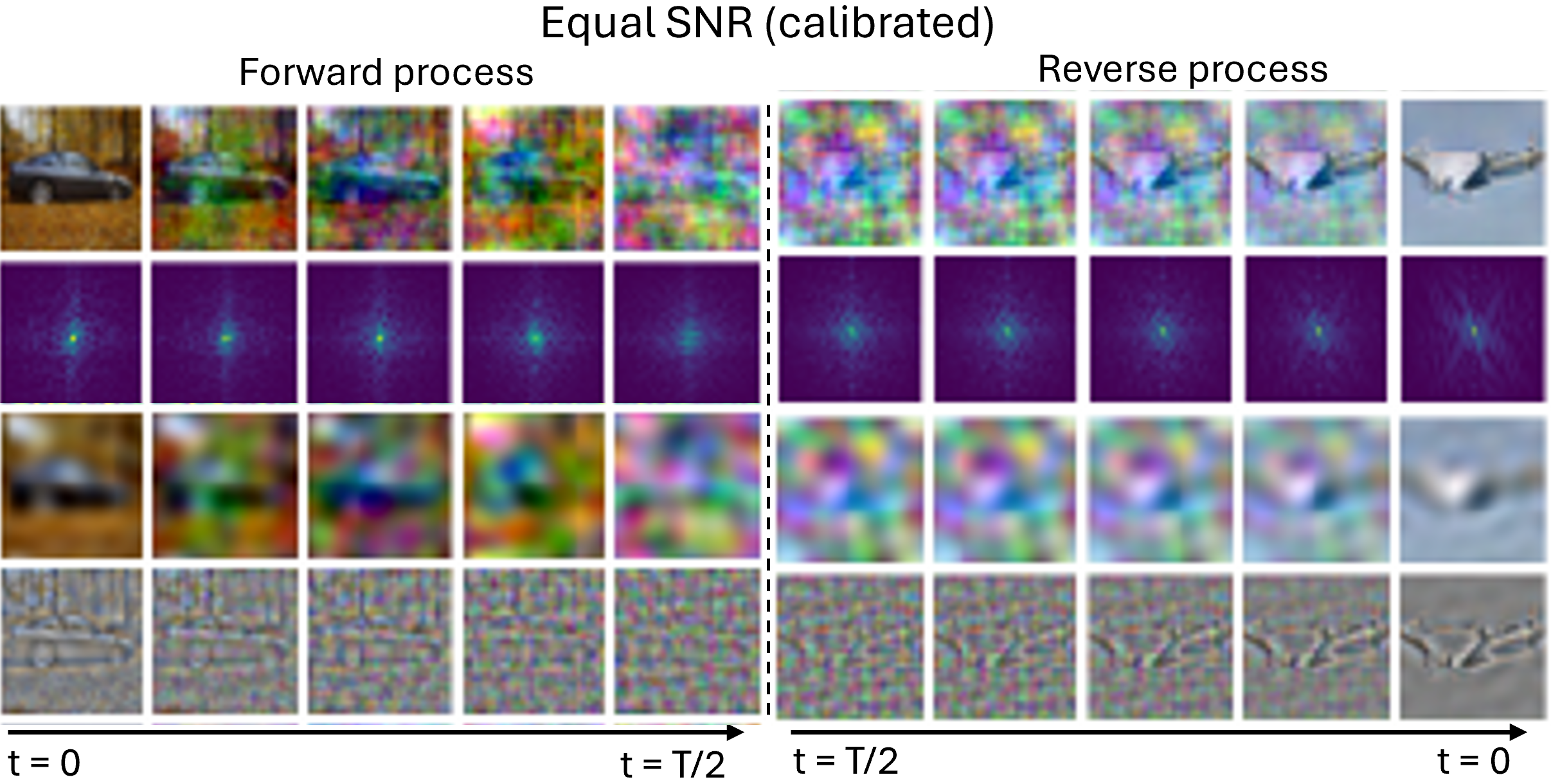
Let’s look at how this forward process qualitatively looks like in Figure 8. We again consider low- and high-pass filtered images during an EqualSNR forward and backward process, complementing the same illustration for DDPM we already looked at. For EqualSNR, both high- and low-frequency information are vanishing all at the same time in the forward process – well, at least sort of. In the reverse process, low- and high-frequencies are likewise being generated at the same rate. Importantly, this diffusion model is hierarchy-free [15]: its frequencies are not generated in a certain order, it is not ‘autoregressive’ or ‘hierarchy-imposing’ in this sense, but the frequency components are generated all at the same time, equally fast.

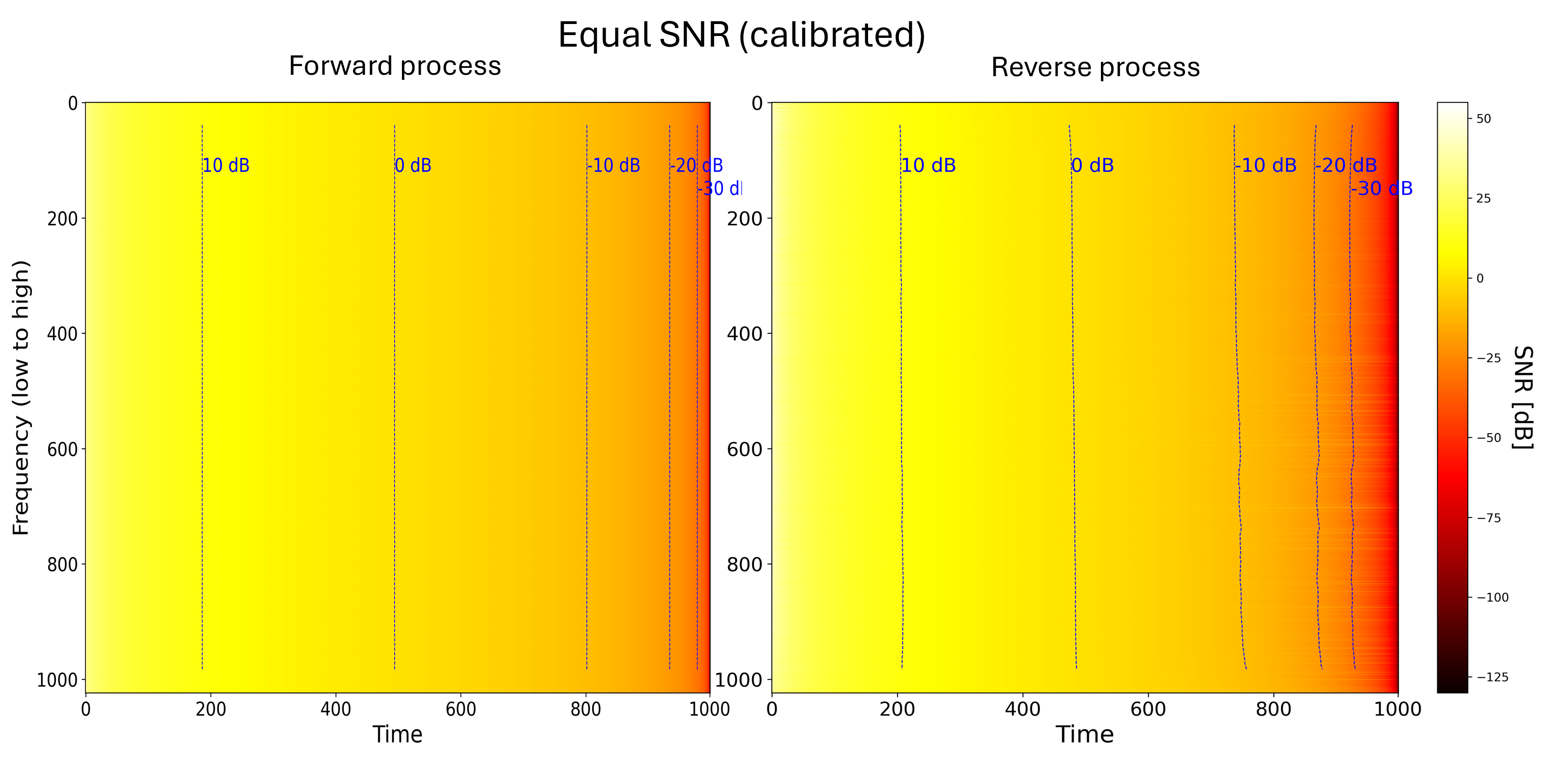
What about quantitatively (Figure 9)? In the forward process, at any time step, the SNR is now equal across all frequencies (by design). Once again, the reverse process mirrors the forward process, as we see from our SNR proxy measure on the right. The diffusion model hence generates all frequencies at the same time, there is no hierarchy or soft ordering among the frequencies anymore.

But what about performance? Can a diffusion model with an EqualSNR noising schedule, even though it is not performing ‘approximate spectral autoregression’, perform as well as a DDPM diffusion model? Perhaps surprisingly to some, the answer is: Yes, it can!

Table 1 shows (Clean-)FID values of diffusion models trained with DDPM and EqualSNR on imaging datasets of different resolution ³. The FID scores are rather comparable between DDPM and EqualSNR. So even though we have no hierarchy in an EqualSNR diffusion model, it works just as well as DDPM. Of course, these results are limited, and would have to be validated with more models and further modalities, too. But what we can conclude is that approximate spectral autoregression is not a necessity. It is an (implicit) choice we made, but other noising schedules with different inductive biases can work just as well.

Fast noising in DDPM deteriorates high-frequency performance

The hierarchy-free EqualSNR forward process seems to perform on par with DDPM, at least for images and looking at Clean-FID. But can it give us any gain? – One advantage is that it can produce better generation quality of high-frequency information, and this is what the paper focuses.

The intuition is very simple: in DDPM, since we add white noise to data which follows a Fourier power law, we not only noise high-frequencies first but also faster, in the sense that per discrete time increment, the SNR for high-frequency components deceases faster than for low-frequency components. As a consequence, the diffusion model spends less timesteps generating high-frequency components. Since the model’s capacity is limited and its weights are shared across all timesteps, high-frequency components have a lower generation quality than low-frequency components, and (I hypothesise that) FID might not capture this.

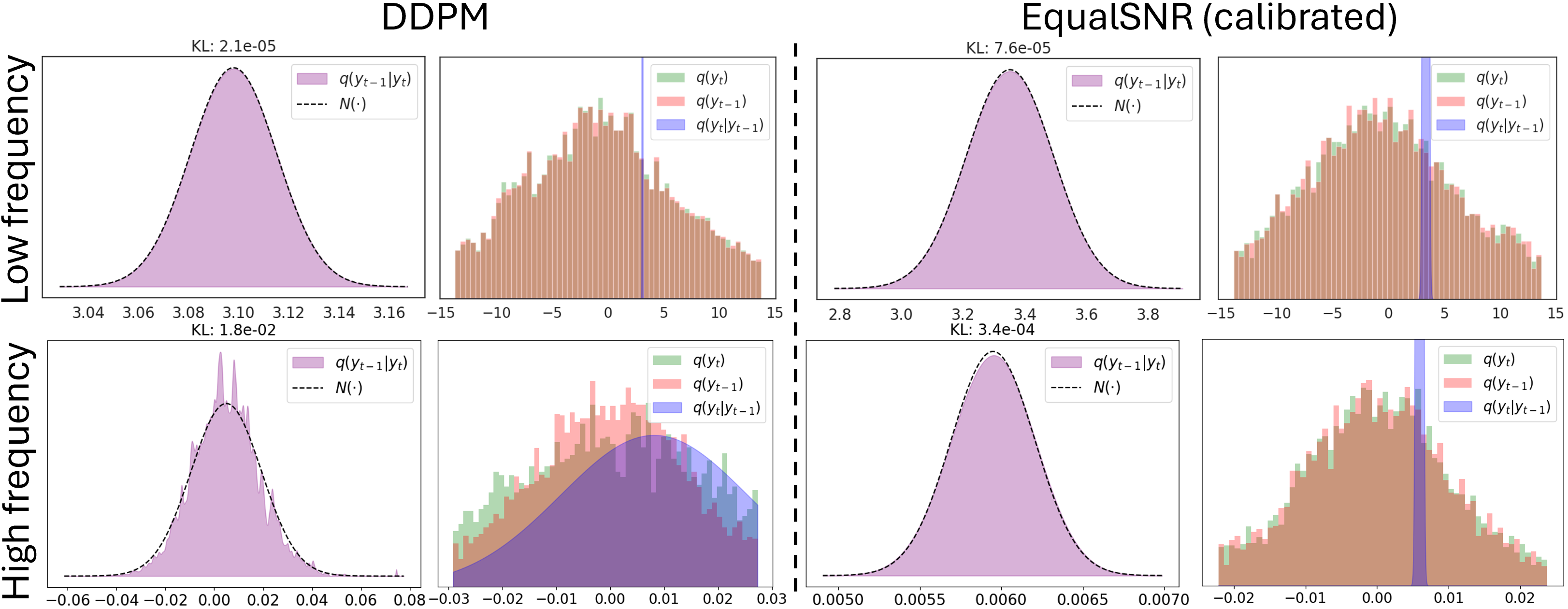
One consequence of the fast noising of high-frequency components is that the Gaussian assumption which DDPM makes on the (intractable) reverse process distribution $q({\mathbf{y}}_{t-1}\mid {\mathbf{y}}_t)$, which $p_{\theta }({\mathbf{y}}_{t-1}|{\mathbf{y}}_t)$ approximates, is violated. This may be a theoretical explanation for lower generation quality of high-frequencies in DDPM.

To see this, we first apply Bayes rule $$q({\mathbf{y}}_{t-1}|{\mathbf{y}}_t)=\frac{q({\mathbf{y}}_t|{\mathbf{y}}_{t-1})q({\mathbf{y}}_{t-1})}{q({\mathbf{y}}_t)}.$$ For high-frequency components, $q({\mathbf{y}}_t|{\mathbf{y}}_{t-1})$ has a large variance relative to $q({\mathbf{y}}_{t-1})$ and $q({\mathbf{y}}_t)$. As a consequence, fluctuations in the quantity $\frac{q({\mathbf{y}}_{t-1})}{q({\mathbf{y}}_t)}$ are more apparent in the distribution $q({\mathbf{y}}_{t-1}|{\mathbf{y}}_t)$. One can formalise this (see Proposition 1 in the paper). Here, I rather want to focus on intuition and illustrate this observation in Figure 10 for a low-frequency [top] and a high-frequency [bottom] for DDPM [left]. Note the spiky⁴ behaviour of the estimate of $q({\mathbf{y}}_{t-1}|{\mathbf{y}}_t)$ in the high frequency, which somewhat deviates from a Gaussian. Since EqualSNR noises all frequencies at the same rate (in terms of SNR), it noises the high-frequencies, which were noised the fastest before, less fast. Consequently, this problematic behaviour does not appear here.

So we would expect that EqualSNR has a better generation quality for high frequencies. To put this to the test, we train two diffusion models, one with a DDPM and one with an EqualSNR forward process, otherwise all things equal (as before). We simulate a dataset where high-frequency information is dominant: black images with a few white pixels (between 46 and 50 to be precise). Now here is the surprising insight: ‘by eye’, we can observe differences in the spectral magnitude profile of generated images contrasting the DDPM and EqualSNR diffusion model. While the EqualSNR model’s spectral magnitude distribution approximately overlaps with the real data distribution, for DDPM, there is a clear deviation in high frequencies, while for low frequencies, the profiles of real and synthetic data roughly overlap. Related work similarly observed that high-frequency generation quality suffers in current diffusion models [29].

Since high-frequency information is dominant in this dataset, we can also observe the impact of this deviation on the quantity of interest, here the number of white pixels. The distribution of white pixels in the generated samples has a mean is shifted and off from the ground-truth number of pixels in the dataset (46 to 50).

In natural images, such differences may not matter, because the human eye cares mostly about getting low frequency information right. But what if we consider data where high-frequency information is key, such as astronomy images, aerial images, or medical images such as MRI? Should we adapt our noising schedules to better accommodate the (high-frequency) data characteristics of such datasets? And what are the implications of (largely) not doing so until now? Furthermore, can we maybe use this insight to detect synthetically generated diffusion samples in the Fourier domain more easily (in the context of watermarking)? And, if we use EqualSNR, might it be harder to detect DeepFakes? – These are some of the questions raised by the paper.

Does any forward process work?

We found that EqualSNR, a schedule with no hierarchical order in Fourier space, works well, even better than DDPM for high-frequency generation. The obvious question to ask is: does any schedule work well, akin to the invariance of the continuos-time loss to the noising schedule?

One thing we tried was to flip the frequency order in DDPM: noise low-frequency components first, and consequently generate high-frequency before low-frequency components. More precisely, this schedule noises the data such that the $i$th frequency has the same SNR as the $D-i$th frequency in DDPM. We call this schedule FlippedSNR, and illustrate it with our usual plot in Figure 11.

Surprisingly, this schedule doesn’t work. I’m not fully sure why, we tried it with a couple of ${\alpha }_t$ schedules and other hyperparameter choices but then moved on. A possible explanation: in FlippedSNR, we noise low frequencies faster than high frequencies, spending less resources on them. Maybe this deteriorates training. Another possible explanation is that maybe the low- to high-frequency is at least partially important: maybe high-frequency information needs at least partial low-frequency information to generate those frequencies efficiently, as is the case in EqualSNR.

Worth highlighting is also the recent work from my collaborators Chris Williams and Saif Syed in Oxford. They derive forward processes which are optimal with respect to a cost that measures the work to transport samples along the diffusion path [30]. Clearly, not any noising schedule works equally well in practice, and their performance can differ a lot.

Closing thoughts

In this blog post, we revisited what approximate spectral autoregression means in DDPM diffusion models, discussed why this might be a beneficial inductive bias, and showed that a hierarchy-free diffusion model, which has no ordering of frequencies and is not approximately autoregressive in Fourier space, works as well as DDPM and even better for high-frequency generation. Most importantly, the preliminary results on images showed that spectral autoregression is perhaps not a necessity for diffusion models to work well.

If it’s not the ordering frequencies, which was induced by the data distributions diffusion models are often used for, what is it that makes diffusion models work well? – Well, that’s the million dollar question. Perhaps it is just the ability of diffusion models to iteratively refine a continuous latent state [31], similar to latent reasoning in LLMs. Since diffusion models use weight-sharing across timesteps, this is a form of self-iteration which I recently explored in the context of LLMs and yields—if one converges towards a fixed-point—performance gains [32]. I don’t have a conclusive answer, and future research will tell.

Thoughts? Ideas? Questions? Feedback? -- I'd love to hear from you!

Citation

If you would like to cite this blog post, you can use:

@misc{falck2025spectralauto,
  author = {Falck, Fabian},
  title = {Diffusion is not necessarily Spectral Autoregression},
  url = {https://fabianfalck.com/posts/spectralauto},
  year = {2025}
}copy

You may also want to cite the paper accompanying this blog post:

@misc{falck2025fourier,
  title = {A Fourier Space Perspective on Diffusion Models},
  author = {Falck, Fabian and Pandeva, Teodora and Zahirnia, Kiarash and Lawrence, Rachel and Turner, Richard E. and Meeds, Edward and Zazo, Javier and Karmalkar, Sushrut},
  url = {https://arxiv.org/abs/2505.11278},
  year = {2025}
}copy

Acknowledgements

I would like to thank my co-authors at Microsoft Research on the paper accompanying this blog post: Teodora Pandeva, Kiarash Zahirnia, Rachel Lawrence, Richard E. Turner, Edward Meeds, Javier Zazo, and Sushrut Karmalkar. They drove this work, and produced and elicited the majority of the thoughts discussed in this blog post.

I would like to acknowledge Sander Dieleman and his blog post Diffusion is spectral autoregression which motivated this blog post. Some of the figures presented above are inspired by him and use the code accompanying the post.

I would also like to thank my colleague Markus Heinonen who I had many interesting conversations with on this and related topics at conferences over the years. The work by Markus and his colleagues inspired Sander’s post, so did it inspire this one.

I would further like to thank my collaborators back at Oxford, particularly Chris Williams and Saif Syed, Matthew Willetts, Chris Holmes and Arnaud Doucet, who I closely worked with during my PhD and where many of the thoughts and questions in this post originate from.

I would like to thank my colleagues Sam Bond-Taylor, Rachel Lawrence, Teodora Pandeva, Ted Meeds and Fernando Pérez-García for proofreading this blog post.

References